Select Calibration Incorporated
Calibration Services for Coordinate Measuring Machines
Calibration
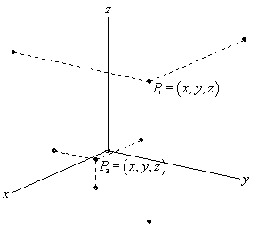
A coordinate measuring machine is a class of equipment designed for three dimensional inspection. These machines provide accurate point data for relative locations within their measurement volume. A typical CMM consists of three axis at right angles to each other (orthogonal) with each axis equipped with a precision scale. Measurements of length are done by finding the coordinate difference between any pair of points in the machine volume and converting this into a 3D distance.
As computers evolved the ability to expand the measurement capability of a CMM has changed significantly. Computers allow the user to combine individual point locations into complex geometric features such as planes, spheres, cones, cylinders, and so on. The geometry allows for additional evaluations such as the angle between the axis of two cylinders or the diameter of a circle. Computers allow the user to record inspection steps into an inspection routine that can be run over and over allowing faster turn around time than what would be possible using traditional methods such as a surface table and height gauge.
CMM's can be manual or motorized. Manual machines are ideal for single part or simple, one time, measurements. Motorized machines are ideal for manufacturing environments where many parts of the same type are produced and sampling is required to monitor the production process. CMM's come in various shapes and sizes and are capable of using a variety of sensors such as hard probes, trigger probes, analogue probes, laser probes, laser scanners, and cameras.
Calibration, in the context of a CMM, is adjusting the machine in order to reduce the relative error between point locations in the machine volume to zero. The purpose of a CMM is one of measuring length where at least two points are required to produce something meaningful. Combining two or more points into geometric features is a variation where the relative positions of the points defines the size, location, and orientation of the measured feature. If there is no relative error between the points in the machine volume then there is no error contribution from the machine.
It is not enough to simply report the current errors of a CMM to the end user particularly if the current errors are large and obvious. For some equipment, such as ring gauges or gauge blocks, knowledge of the actual length or size of the artifact is information that is actually usable but this doesn't really work on a CMM as machine errors are almost impossible to subtract from measurements performed using the machine. At best, in this situation, the measurement uncertainty from using the CMM would need to be set high enough to contain all the known machine errors. This is the primary reason that Select Calibration Incorporated does not perform verification only calibrations of CMM's as this is not the expectation of the end user.
Calibration of a coordinate measuring machine is surprisingly complex. Removing known errors of the machine can be done by mechanical adjustments or through software. Software adjustment is something that is needed when the limits of mechanical adjustment has been reached or is not possible. Over time almost all manufacturers had adopted a nearly identical process of describing basic geometry errors of the individual axis and using this to apply software correction at a level that is hidden from the user.
Most coordinate measuring machines have 21 calibration map parameters that can be adjusted through software. A minimum set of calibration map parameters would be scale factors and squareness. Some machines have compensation parameters to deal with problems such as: deflection errors for horizontal arm CMM's, axis with two or more scales, hysteresis errors, shape changes from part weight that is placed on the machine, or shape changes in the machine due to changes in temperature. Machines with parametric temperature compensation can have up to 42 compensation parameters active at any one time (21 static parameters and 21 dynamic parameters based on sensitivity to temperature) which adds a good deal of complexity to something that is already complex.
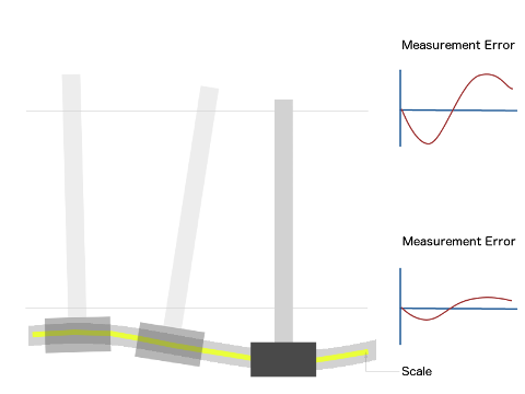
A good indication that the machine calibration is correct is when the axis moves at the proper increment in a straight line both horizontally and vertically. Observed straightness errors is a good indication that one or more angular problems exist. Unusual shape errors in the scale are typically a product of angular problems as measurements are never performed directly at the position of the scale. Mechanically accurate machines will have very little angular, straightness, and scale shape errors while software compensated machines with significant angular errors will show predictable amounts of scale and straightness errors.
Calibration of a three axis CMM is far more involved then simply comparing each machine axis to a reference standard. For a three axis machine a twist or bend in any one axis will directly affect the axis that follow in the kinematic chain. The effects from twists and bends will change as you move throughout the machine volume requiring a valid look-up table of corrections depending on where the machine is located.
Manufacturers minimize accuracy related problems as much as possible by using materials and processes that produce bearing guide-ways with minimal twisting and bending. Mechanically producing a perfect machine is either impossible or impractical due to the costs involved. Residual errors from manufacturing are removed from the machine by software which uses the data from the compensation map as the basis of correction.
In order to properly calibrate a CMM it is important to inspect and update all geometry errors from each axis. Some machines are quite stable and will change very little over time while others will change shape from thermal cycling over the course of its lifespan. All machines require periodic updates to ensure the best measurement performance possible.
Compensation maps are an essential part of most CMM's and allows for adjustments that can be very difficult, if not impossible, to perform by only mechanical means. Most manufactures of modern CMM's rely on the compensation map to achieve the target performance whereas the very best machines use a combination of good mechanical design and software compensation.
Temperature compensation is an attempt to minimize the errors of a machine due to changes in temperature. As temperature changes the material used to construct the CMM will grow or shrink, twist, and bend. Since the machine structures are complex shapes with welded reinforcements throughout the change in shape is difficult to predict. For this reason it is always preferred to have the machine in a proper thermal environment over relying on temperature compensation.
All measurements are reported with the expectation that the result is what was found at 20 C. If the environment is not at 20 C then it is necessary to account for any expansion of the part and machine so that the end result is the expected result at 20 C. Due to the unknowns of the CMM axis expansion coefficient and, more critically, the part expansion coefficient, measurements at temperatures other than 20 C contribute to the measurement uncertainty.
One type of temperature compensation that can be used on a machine is simple scale correction for each axis and the part. Each axis of the machine has a known expansion coefficient and will grow and shrink by an expected amount. The part expansion coefficient can be estimated by knowing the material of the part and referring to established values. This kind of temperature compensation does not take into account changes in the shape of the machine or the part but only the expected change in the machine scales and part as a simple linear correction.
Another type of temperature compensation involves actively changing the amount of software compensation applied to the CMM as the temperature changes. Each family of machines that use this type of compensation will undergo testing in an environmental chamber in order to produce the required correction coefficients based on where the changes in shape are occurring. The correction can be either a complex curve or a simple gradient depending on which compensation map parameter the correction is applied to.
For CMM's that use temperature compensation, particularly models with full parametric compensation, it is necessary to take this into account when performing a calibration. The physical machine error will be the sum of the error described in the compensation map from the reference temperature and the expected change in shape at the current measurement temperature.
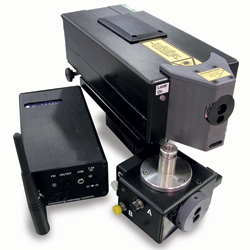
Select Calibration Incorporated uses a combination of special hardware and software to collect and apply compensation data. The technology exists to collect all compensation parameters simultaneously and, when combined with custom software to process the raw measurement data, a CMM axis can be completely re-mapped in as little as one measurement cycle. The compensation parameters collected from the laser are roll, pitch, yaw, horizontal straightness, vertical straightness, and the scale error.
The preferred method for data collection is by direct measurements which is the method used by Select Calibration Incorporated. Using equipment such as Laser Trackers to map a machine volume is an example of indirect measurements. Indirect measurement data collection using a Laser Tracker is effective but it relies on fitting measurement lines from several points of view in the machine volume and then guessing at the source of the error (called the Monty Carlo method). A Laser Tracker should not be used in place of traditional lasers as they are not accurate enough unless the Laser Tracker is used in an overlapping data collection pattern with measurements from multiple points in the machine volume and using only the distance measurement data from the laser for updates.
Data collection using traditional lasers is good but it is a slow process. When using a traditional laser each compensation map parameter requires a separate setup and measurement independent of every other compensation map parameter. Collecting the standard six sets of measurement data for an axis will require six measurement setups and six measurement cycles of the machine. If, for example, the setup time is 20 minutes for each parameter and the measurement cycle takes 20 minutes then one axis can be re-mapped in approximately 4 hours (6 parameters, 20 + 20 min for each). When using a laser that can collect all compensation parameters simultaneously the calibration time is reduced to 40 minutes. The advantage of using a multi-parameter laser becomes obvious in this context.
Completely re-mapping a CMM axis eliminates the need to perform initial investigative measurements to determine which compensation map parameters require updating and which ones can be ignored. Since all compensation map parameters are updated the investigative testing is redundant. Data collection with traditional lasers is quite laborious so to reduce the amount of time investigative measurements are usually done in order to plan the measurement strategy instead of simply measuring everything.
Unattended or automated data collection is used in all cases where possible. There are several advantages of automated data collection most notably that the data collection is consistent where every single data point is measured in the exact same manor as every other data point. Automated data collection is preferred in less than ideal environments where many measurements can be performed with no additional effort by the technician performing the tests.
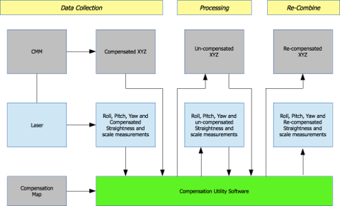
The Map2Map Compensation Processor software is at the heart of the ability to remap a CMM axis in a single measurement cycle. This software calculates the residual errors from changes in the compensation data while taking into account effects from parametric compensation. Without this unique software single cycle data collection would not be possible.
The most commonly overlooked problem when capturing measurement data during a CMM calibration is the handling of the measurement data. For a machine that has only 10 measurement positions per axis the results would still be 180 data entry values that must be handled (10 positions x 6 parameters x 3 axis = 180). Manual entry is often used to transport data between incompatible software when this problem has not been considered or has been ignored. To eliminate data entry errors and reduce the calibration time a variety of tools have been developed to transport and process measurement data directly from the equipment to the compensation map. With rare exception most equipment software can provide data by either file or through direct communication with the target device.
Testing is necessary in order to prove the coordinate measuring machine is measuring properly.
Standards exist so that comparison of values is possible between different individuals or organizations. Without standards, or at least a full understanding of how a particular value was derived, measurement results would be meaningless and not comparable. It would be the same as stating something like “the result of Test A was 0.0034 mm and the result from Test B was 0.0058 + 0.0034L mm” but without knowledge of what Test A and Test B are the results have no meaning and could not be reproduced by anyone other than the organization who originally performed those tests.
Select Calibration Incorporated follows the ASME B89.4.10360 or ISO/IEC 10360 family of standards for performance evaluation of coordinate measuring machines. The 10360 family of standards is titled Acceptance and Reverification Tests for Coordinate Measuring Machines and contains the following sub sections:
The predecessor to the ASME B89.4.10360 standard is ASME B89.4.1 (ball bar). This is an obsolete standard and has been replaced by ASME B89.4.10360-2:2008. It was decided not to offer CMM calibrations that include the use of a ball bar for performance testing because investing resources in this obsolete standard does not make sense.
The following sections list some of the performances tests from the 10360 family of standards.
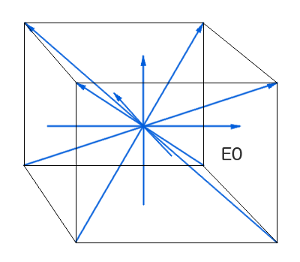
This test is the measurement of 105 lengths performed in seven specified directions with each measurement direction consisting of five lengths measured three times. Each individual length from the 105 results is compared to the specification (no averages are used). The probe used to perform this test should have a zero or minimal probe offset perpendicular to the ram axis of the CMM.
Criteria for strict acceptance is that all of the 105 individual lengths must have a deviation from nominal that is less than the manufacturer specification reduced by the expanded uncertainty.
Results are usually displayed graphically where the length deviations can be visually compared to the specification. The specification is length dependent and forms a funnel shape around the nominal.
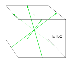
This test is the measurement of 30 lengths performed in either the YZ or ZX measurement planes. A single direction (not shown in image) can be used if performed by diametrically opposing probes otherwise two directions are required. Each direction consists of five lengths measured three times. Each individual length from the 30 results is compared to the specification (no averages are used). The probe used to perform this test must have an offset of 150 mm perpendicular to the ram axis of the CMM.
Criteria for strict acceptance is that all of the 30 individual lengths must have a deviation from nominal that is less than the manufacturer specification reduced by the expanded uncertainty.
Results are usually displayed graphically where the length deviations can be visually compared to the specification. The specification is length dependent and forms a funnel shape around the nominal.
This test of repeatability is not a separate test but a derived result from the E0 measurements. For each of the 35 sets of three repeated length measurements the range of the length results are found. Criteria for strict acceptance is that all 35 sets of repeatability ranges must be less than the manufacturers specification reduced by the expanded uncertainty.
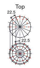
This test is a measurement consisting of 25 defined points on a precision sphere. The least squares center of the sphere is found from the 25 points and, for each of the points, the radial distance is calculated from the center of the sphere. The probing error, PFTU, is the difference between the maximum and minimum radial distance.
Criteria for strict acceptance is that the range from the maximum to minimum radial distance must be less less than the manufacturer specification reduced by the expanded uncertainty.
Note: This test was part of ISO/IEC 10360-2:2001 standard but was removed from the 2009 version and is now part of ISO/IEC 10360-5:2010.
Uncertainty in measurement represents the variability for any reported value based on incomplete knowledge of the measurement. The final uncertainty value represents the sum of the unknown errors accumulated between the transfer standards and any contribution from the measurement the uncertainty value is associated with.
In reference to length the definition of a meter by the international system of units is the distance that light travels in 1/299,792,458 seconds. Only a few artifacts are actually measured against the speed of light since the equipment and expertise needed to perform this measurement accurately would become very expensive and can likely only be performed by a national measurement institute such as NRC or NIST. The artifacts that are calibrated by the top level national institutes are used as transfer standards to measure additional artifacts which are then used to calibrate other artifacts and eventually to the level of the working standard such as a gauge block.
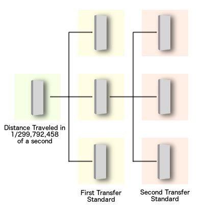
Each measurement transfer can contribute an unknown amount of measurement error. Each artifact has imperfections that may not be fully understood at the time of measurement. The equipment used to perform the comparison between the known and unknown also has imperfections that can affect the results. This grey area is considered to be a potential error that may or may not exist and represents the uncertainty.
The number of intermediate transfer standards between the primary and the working standard affects the amount of potential error or uncertainty. This system provides a way to ensure that circular calibration does not occur where one company calibrates the artifacts for a second company that in turn calibrates the artifacts for the first company in an isolated manor. If uncertainty is properly considered at each step eventually the uncertainty in this situation will grow beyond reasonable values.
Some confuse measurement repeatability with measurement uncertainty. Measurement repeatability provides an idea of variability but cannot take into account the deviation from the true value. Measurement repeatability is only a contributing factor to measurement uncertainty.
Traceability as defined by NIST: "Traceability of measurement requires the establishment of an unbroken chain of comparisons to stated references each with a stated uncertainty.".
There are several requirements to produce a traceable measurement. The biggest one is that a measurement must be performed by an organization that is competent and recognized to do so. Accreditation to ISO/IEC 17025 or an equivalent standard with the measurement discipline listed on the accreditation scope is a requirement for a traceable measurement.
In addition to recognition a reasonable estimation of the contribution of measurement uncertainty must be produced. This uncertainty value will contribute to the chain of uncertainties back to the definition of the measurement unit by the international system of units. If a calibration is performed by a company who is not recognized to perform this work then the results, and any subsequent results, are no longer considered traceable to the SI units.
In order to assign an uncertainty value to a measurement it is necessary to understand and list all the contributing errors associated with the measurement and assign a value to each. The unknown part of the measurement cannot be determined directly (it would no longer be considered an unknown if it can be determined) but it can be estimated by considering at all the sources that contribute to potential error. This list of error sources and contribution values, when properly organized, is referred to as an uncertainty budget.
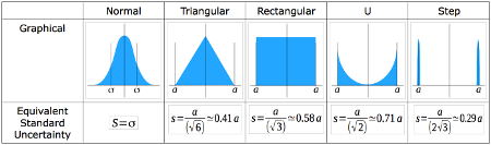
The contribution from each value in the uncertainty budget is in the form of a standard uncertainty. A standard uncertainty is comparable to a standard deviation for a given set of data. The conversion to a standard uncertainty from a potential error source is done based on the distribution type and range associated with the value. For example, a standard uncertainty from a non-normal (rectangular) distribution of some range could be converted to a standard uncertainty by dividing the range with the constant 1.73.
The type of contributing uncertainty can either be A or B. Type A sources are from direct measurements such as repeatability. Type B sources are values where only basic information is known about the source such as the resolution of the measurement instrument or calibration uncertainty of the reference artifacts used for the measurement.
All sources in the uncertainty budget should be listed even if the influence is very small or negligible. Large uncertainty sources that has little effect on the specific measurement can be handled by setting a sensitivity value reflecting the amount of influence it has on the measurement. Listing items that contribute only a small amount to the total uncertainty at least acknowledges that the contribution has been considered.
The total uncertainty is calculated as the square root of the sum of the squares for each uncertainty component as described by GUM.
The reported uncertainty on the calibration report is the standard uncertainty calculated from the uncertainty budget expanded to a desired coverage level. The coverage describes the number of standard uncertainties is represented by the uncertainty value. A coverage value of 1 would represent 68% of the total range whereas a coverage of 2 means that the uncertainty represents two standard uncertainties or 95% of the total range and 3 represents 99% of the total. The most common coverage value used is 2 and will appear as (k=2) on the calibration report.
In order to provide a good estimate for measurement uncertainty when calibrating CMM's a couple of problems need to be solved. One important problem is that the calibration is always performed onsite and many of the contributing uncertainty sources change from site to site. For example, environmental conditions are frequently different between different customers which potentially has the largest impact on the final measurement uncertainty. Individual machines can have differences such as scale resolution, type of probing, and even repeatability characteristics that can have an impact on measurement uncertainty. The selection of equipment used for testing by the calibration service provider will also contribute to the final measurement uncertainty. Uncertainty budgets, especially when dealing with a variety of CMM's for different customers, takes on the form of an abstract list of error sources that cannot be estimated in advance.
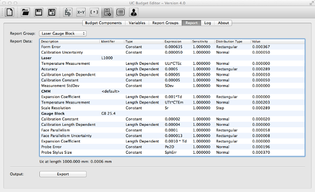
The solution used by Select Calibration Incorporated for this problem is to use a dynamically calculated uncertainty budget. Instead of assigning constants to the uncertainty budget each value is treated as an expression with variables. The variables represent the different aspects of the machine, environment, and selected equipment along with anything else that can change from machine to machine. For example, consider the scale resolution. The uncertainty from a scale with a resolution of 0.001 mm is calculated by one of these two methods (both results are identical but written differently depending on interpretation):
Instead of using the static constant of 0.001 in the uncertainty budget an expression with the variable Sr is used to represent the contribution from the scale resolution. The expression would end up looking like this:
When moving from machine to machine only the variable information describing the scale resolution needs to be provided which would automatically update this component and all related components.
In addition to the scale resolution, variables can be used for temperature deviation from the nominal, temperature gradient, uncertainty of the expansion coefficient of machine and equipment, uncertainty of the selected probe error, uncertainty of the calibration equipment such as the thermometer, step gauges, gauge blocks, laser, and any other items that vary from machine to machine. The measurement uncertainty is automatically calculated when a calibration report is generated. The uncertainty budget used by Select Calibration Incorporated has seamless integration with the reporting software. The reported uncertainty value using this setup is almost always unique to the customer.
Uncertainty expressions is a description of the measurement uncertainty expressed as a formula such as Uc = A + Bx. The measurement uncertainty for any given length would be determined by substituting the length of the measurement into the equation to produce a single value.
The calibration reports issued by Select Calibration Incorporated do not use uncertainty expressions but instead show a single uncertainty value attached to each measured result. It was decided to use this method instead of an uncertainty expression in order eliminate approximation errors.
The scope of accreditation for Select Calibration Incorporated uses expressions to represent the uncertainty over an unspecified length. The uncertainty expressions used by Select Calibration Incorporated include both constant and length dependent components in the format Uc = A + Bx + Cx^2. Using a curve fit of the uncertainty data provides a more realistic representation as compared to a line fit of the same data. The following shows an example of the why a curve fit of the uncertainty expression is used and not a simple line fit:
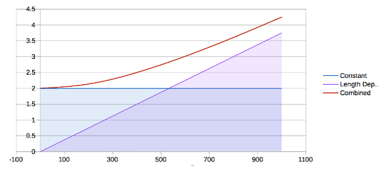 |
Contribution from all sources listed in the uncertainty budget with the constant and length dependent components shown in different solid colors. The combined value from the constant and length dependent components produce a curve. |
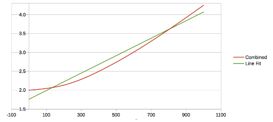 |
Result of using a best fit line to describe the curved shape of the uncertainty data. The biggest concern with this is that the line at length zero (y intercept) is almost always lower than what could potentially be achievable by the laboratory. In some cases this value may be negative if the curve is pronounced enough. |
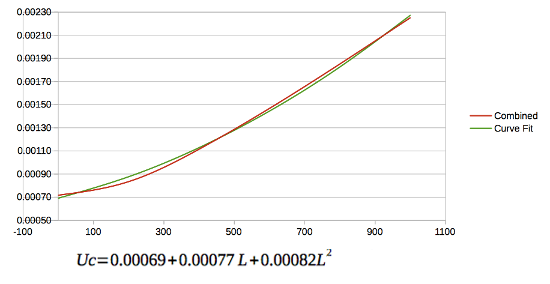 |
Comparison of actual uncertainty data calculated at different lengths as compared to the best fit curve uncertainty expression. Although the fit is not perfect it is much better at describing the real shape then what would be possible using only a line. The expression used to generate the shape is displayed below the graph with L representing the position in meters. |